I mentioned in a previous blog an Excel Intermediate course where some delegates who used Excel all day every day did not know how to enter a formula to calculate a simple multiplication. But practically everyone has come across the AutoSum button on the Home tab of the Ribbon.

Excel's Help topic states that the easiest way to add a SUM formula to your worksheet is to use the AutoSum Wizard. Select an empty cell directly above or below the range that you want to sum, and on the Home or Formula tabs on the Ribbon, click AutoSum. The AutoSum Wizard will automatically sense the range to be summed and build the formula for you. It can also work horizontally if you select a cell to the left or right of the range to be summed.
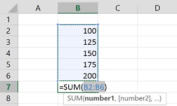
So here is an example of how this works. We have values in cells B2 through B6 that we want to sum so we selected B7 below these values and clicked AutoSum. The AutoSum Wizard has automatically sensed the range B2:B6 and supplied this argument to the SUM function. Pressing Enter or clicking AutoSum again will enter the formula in cell B7 for us.
Marvellous! Who needs to know anything about entering and editing formulae when Excel will do all the work for you?! But the AutoSum Wizard is not infallible and may not always give you the answer you are expecting, as in the example below.
Here we have some data for the previous five years and we want to a total for each year. We can select where we want the totals and then quickly enter the SUM function by one click of the AutoSum button.
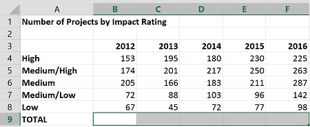
Rather than pausing to display the suggested range, with a multiple selection Excel immediately puts the SUM function into each cell, adding together the data directly above for each column.
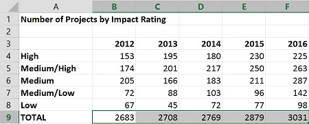
Do those results look right to you? Are they not a bit on the high side? Excel has automatically included the year "headings". They are headings to us but to Excel they are values.
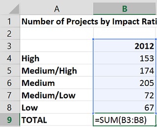
So, we can edit the formula to make the range B4:B8 to avoid the headings, and then Excel displays the error indicators to tell us that the formula omits adjacent cells!
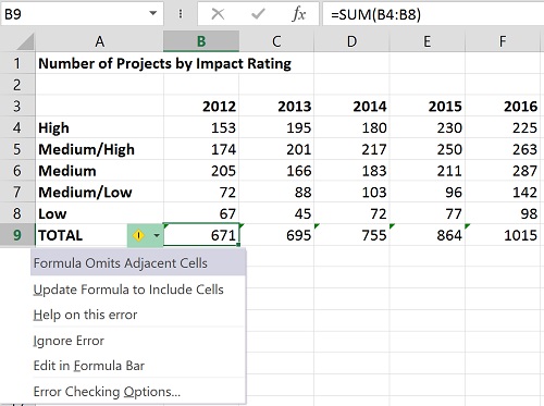
In this instance it is Excel who has – unwittingly – made the error and we can tell it to ignore the error or just live with the little green triangles showing on the screen (they don't print).
But of course, on other occasions the error indicators may be legitimately warning of a problem. And there are numerous ways of getting AutoSum to use the range of cells you want by having a deeper understanding of how it works and selecting cells and ranges appropriately.
ONE TIP: You can use ALT+ = to quickly add the SUM function to a cell with an empty argument – =SUM(|). Then you can type or select your range(s) manually.
What this all goes to show is that Excel is not always as clever and helpful as you may think and it is vitally important to check your formulae and results.
So many organisations depend heavily on Excel spreadsheets for crucial calculations and analysis. Are you confident of the validity of your spreadsheets? We can run a training session or workshop to cover some of the techniques that you can use to make your spreadsheets accurate and robust. Get in touch for more details.

